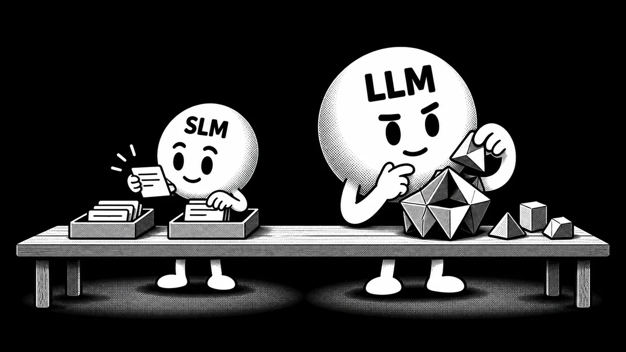

Do you need a large language model (LLM) or does a small language model (SLM) suffice for your task? At what point does running an SLM become not enough? And what does SLM even mean? We tested small language models vs large language models on the same hardware to answer these questions.
Quick answer
The quality gap between SLMs and LLMs is relatively small on routine, well-defined tasks. In our LLM vs. SLM test, a 1.45 GiB model scored within 6.5 percentage points of a 15.33 GiB model on routine work, but the gap widened sharply on extraction, coding, and multi-constraint instructions.
What Is a Small Language Model (SLM)?
A Small Language Model (SLM) is an AI language model designed to perform many of the same tasks as a large language model (LLM), but with far fewer parameters and lower computing requirements.
SLM is a loose term. While an LLM may contain tens or hundreds of billions of parameters, an SLM may have anywhere from hundreds of millions to several billion. For example, Lu et al. classify SLMs as models with 100 million to 5 billion parameters, while Gupta et al. survey SLMs in the 1-8 billion parameter range. Wang et al. explicitly note that some studies classify models with up to 10 billion parameters as small. As a rough rule of thumb:
- Tiny models have under 1 billion parameters
- Typical SLMs have ~1-7 billion parameters
- Larger SLMs have ~7-10+ billion parameters
SLMs are especially useful for local inference as they can run faster, and on smaller hardware, including laptops and mobile devices.
For example, a 2025 position paper, Small Language Models are the Future of Agentic AI, makes a case for assigning repetitive, specialized calls to smaller models instead of invoking a general-purpose LLM every time.
Examples of SLMs include:
| Model | Parameter Count |
|---|---|
| Qwen3-4B | 4B |
| SmolLM3-3B | 3B |
| Gemma 3 4B IT | 4B |
| Phi-4-mini-instruct | 3.8B |
| Llama 3.2 3B Instruct | 3B |
What Is a Large Language Model (LLM), as opposed to SLM?
As opposed to an SLM, a large language model (LLM) generally refers to a language model with billions, or, under some definitions, tens of billions, of parameters.
As we said above, SLM vs LLM is a loose classification, and there is no universally accepted parameter threshold separating SLMs from LLMs.
For example, Minaee et al. describe prominent LLMs as having tens to hundreds of billions of parameters, whereas Zhao et al. describe LLMs more broadly as models with at least several billion parameters.
As a general rule of thumb: models with 3B, 4B, or 7B parameters can be described as SLMs. A 70B model would normally be described as an LLM. Models that have around 12B-20B are sometimes classified as SLMs and sometimes as LLMs.
Key Differences Between Small and Large Language Models
Quality on Simple and Complex Tasks
For simple, well-defined tasks, an SLM can perform surprisingly close to a much larger model. The gap becomes more important when a task requires several operations at once.
For example, in our tests, MiniCPM5-2B Q4 scored 0.932 across 62 routine tasks, compared with 0.997 for Qwen3.8-27B Q4. On the more difficult set, however, their scores fell to 0.560 and 0.734 respectively. The difference was especially large in dirty extraction, where the models had to normalize data and perform arithmetic: 0.29 versus 0.78.
| Test | MiniCPM 2B | Qwen 27B | SLM result |
|---|---|---|---|
| Routine tasks | 0.932 | 0.997 | 93.5% of Qwen's score |
| Difficult tasks | 0.560 | 0.734 | 76.3% of Qwen's score |
| Dirty extraction | 0.29 | 0.78 | 37.2% of Qwen's score |
The practical difference is therefore small on routine work but much larger on tasks that combine reasoning, transformation, and strict requirements.
Size is not the only factor either. LFM2.5-2.6B Q4 scored 0.729 on our difficult set, almost matching the 27B Qwen at 0.734, 99.3% of its score. LFM was the only model whose reasoning could not be disabled, so we gave it a 10× token budget. This comparison therefore reflects the configurations as tested: parameter count alone does not predict task quality.
Memory Requirements and Quantization
Language model memory requirements depend on more than parameter count. Smaller models generally need less memory, which makes them easier to run on laptops, consumer GPUs, and other constrained hardware. But context length and architecture can change that advantage substantially.
In our measurements, MiniCPM5-2B Q4 used 2,188 MiB of VRAM at a 4k context and 7,520 MiB at 128k. That is a 3.4× increase. At 128k, the 2B MiniCPM actually used 32% more VRAM than the 9B Ornith model used at 4k.
| Comparison | VRAM |
|---|---|
| MiniCPM 2B, 4k context | 2,188 MiB |
| MiniCPM 2B, 128k context | 7,520 MiB |
| Ornith 9B, 4k context | 5,714 MiB |
Architecture also changes how quickly memory use grows with context. Between 4k and 128k, MiniCPM added 5,332 MiB of VRAM, while LFM2.5-2.6B added only 2,108 MiB. MiniCPM's increase was therefore about 2.5× larger, despite the models being similar in parameter count.
Quantization can further reduce the memory needed for model weights and make larger models practical on limited hardware. In practice, parameter count gives you a useful starting point, but context length, architecture, and quantization determine what will actually fit.
Speed and Response Time
SLMs are usually faster because they require less computation for each generated token. That advantage matters for interactive applications, high-volume workloads, and local inference.
In our test, MiniCPM5-2B Q4 generated 485 tokens per second, compared with 79 for Qwen3.8-27B Q4, 6.1× the decoding throughput. It also returned the first token from a 9k-token prompt in 0.39 seconds instead of 2.61 seconds, about 6.7× sooner.
| Metric | MiniCPM 2B | Qwen 27B | SLM advantage |
|---|---|---|---|
| Generation speed | 485 tok/s | 79 tok/s | 6.1× faster |
| Time to first token, 9k prompt | 0.39 s | 2.61 s | 6.7× sooner |
Raw tokens per second do not always translate into a faster completed task, however. LFM2.5-2.6B reached 537 tokens per second but generated 325 tokens for a classification prompt that other models answered in two. Its answer therefore took longer despite its higher generation speed.
So for practical comparisons, look at total response time and response length alongside raw generation speed.
Dense Models and MoE Models
Parameter count becomes less straightforward with mixture-of-experts (MoE) models, where active vs total parameters is the distinction that matters. A dense model uses all of its model parameters for each token, while an MoE model activates only a subset of its experts. This lets an MoE model combine the storage footprint of a large model with some of the compute characteristics of a much smaller one.
Ornith-1.5-35B-A3B is a good example. It has roughly 35B parameters in total but activates about 3B for each token. In our tests, it generated 287 tokens per second, compared with 79 for the dense Qwen3.8-27B, about 3.6× the throughput.
However, Ornith used 20,780 MiB (20.29 GiB) of VRAM at a 4k context, the highest 4k-context VRAM use in our test. In other words, 3B active parameters made it fast, but 35B total parameters still made it large to store and run.
We tested Small vs Large Models
We tested nine model configurations on the same hardware and with the same inference setup. The machine used an NVIDIA RTX PRO 6000 Blackwell Workstation Edition with 96 GB of VRAM, 28 vCPUs, 125 GB of system RAM, and Ubuntu 24.04. We ran the current mainline llama.cpp, built with CUDA support for the Blackwell architecture.
For the LLM vs SLM quality comparison, we focused on two kinds of work.
- Routine, structured work where smaller models are often considered a practical alternative to LLMs: classification, extraction, format conversion, grounded question answering, and rewriting.
- The second deliberately made those tasks harder by adding messy inputs, calculations, strict factual requirements, executable code, or multiple simultaneous instructions.
This let us measure not only whether an SLM could handle a task, but also where the gap to a larger model started to widen.
The routine set contained 62 tasks: 24 ticket classifications, 10 invoice extractions, 8 format conversions, 12 questions answered strictly from supplied text, and 8 constrained rewrites. The difficult set contained 12 tasks, with three each for dirty extraction, fact-controlled summarization, standard-library coding with unit tests, and instruction following with six to eight simultaneous constraints.
Each model received the same prompt byte for byte. Quality tests used a 16k context, batch size 1, temperature 0, seed 1234, FP16 KV cache, and no speculative decoding. We disabled reasoning wherever the model allowed it. LFM2.5-2.6B was the exception: neither the server flag nor enable_thinking: false stopped its reasoning, so we gave it a 10× token budget to allow a final answer to emerge.
In total, the quality pass produced 666 scored answers, calculated programmatically.
Test results
Each task score is normalized from 0 to 1, where 1 means that every automated check passed. Aggregate scores are the mean across all tasks in the set, so task groups contribute in proportion to their number of test cases.
The two bold columns summarize different levels of difficulty: Everyday combines the five routine task groups, while Complex combines dirty extraction, controlled summarization, tested code, and multi-constraint instructions. The remaining columns show which task types drive those totals, since two models with similar overall scores may still fail on different kinds of work.
| Configuration | File, GiB | Everyday | Complex | Classify | Extract | Convert | Grounded QA | Rewrite | Dirty extract | Summarize | Code | Instructions |
|---|---|---|---|---|---|---|---|---|---|---|---|---|
| MiniCPM5-2B Q4 | 1.45 | 0.932 | 0.560 | 0.96 | 0.98 | 0.83 | 0.92 | 0.92 | 0.29 | 0.84 | 0.52 | 0.59 |
| LFM2.5-2.6B Q4 | 1.56 | 0.932 | 0.729 | 1.00 | 0.98 | 0.88 | 0.75 | 1.00 | 0.92 | 1.00 | 0.33 | 0.67 |
| Spark-X2.5-4B Q4 | 2.42 | 0.945 | 0.597 | 0.96 | 0.96 | 0.75 | 1.00 | 1.00 | 0.44 | 0.90 | 0.53 | 0.52 |
| Ornith-1.5-9B Q4 | 5.38 | 0.991 | 0.633 | 1.00 | 0.98 | 1.00 | 1.00 | 0.96 | 0.44 | 0.80 | 0.62 | 0.67 |
| Qwen3.8-27B Q4 | 15.33 | 0.997 | 0.734 | 1.00 | 0.98 | 1.00 | 1.00 | 1.00 | 0.78 | 0.80 | 0.73 | 0.62 |
| Ornith-1.5-35B-A3B Q4 | 20.22 | 0.968 | 0.605 | 0.92 | 1.00 | 1.00 | 1.00 | 1.00 | 0.36 | 0.80 | 0.62 | 0.64 |
| MiniCPM5-2B Q8 | 2.50 | 0.900 | 0.601 | 0.92 | 0.98 | 0.71 | 0.92 | 0.92 | 0.44 | 0.87 | 0.47 | 0.62 |
| Ornith-1.5-9B Q8 | 9.11 | 0.997 | 0.666 | 1.00 | 0.98 | 1.00 | 1.00 | 1.00 | 0.44 | 0.93 | 0.62 | 0.67 |
| Qwen3.8-27B Q2 | 9.15 | 0.984 | 0.738 | 1.00 | 1.00 | 1.00 | 0.92 | 1.00 | 0.69 | 0.90 | 0.73 | 0.62 |
The difference was less pronounced on routine tasks: MiniCPM5-2B Q4 reached 0.932, close to Qwen3.8-27B Q4 at 0.997 despite being much smaller.
On the complex set, MiniCPM5-2B Q4 and Qwen3.8-27B Q4 were further apart: 0.560 versus 0.734.
Speed, memory, load time, and energy
We measured performance in a separate sequential pass with only one model occupying the GPU.
The prefill column shows how quickly the model reads a prompt, while generation speed measures how quickly it produces the answer. We also measured time to first token after a 9k-token prompt and sampled power use at 5 Hz throughout a complete ticket-classification response.
| Configuration | File, GiB | Load, s | Prefill, tok/s | Generate, tok/s | VRAM 4k, MiB | VRAM 32k, MiB | VRAM 128k, MiB | TTFT 9k, s | J/task |
|---|---|---|---|---|---|---|---|---|---|
| MiniCPM5-2B Q4 | 1.45 | 1.04 | 24,909 | 485 | 2,188 | 3,392 | 7,520 | 0.39 | 67 |
| LFM2.5-2.6B Q4 | 1.56 | 2.00 | 28,399 | 537 | 2,354 | 2,830 | 4,462 | No answer | 265 |
| Spark-X2.5-4B Q4 | 2.42 | 2.00 | 17,911 | 335 | 3,426 | 4,462 | 8,014 | 0.57 | 118 |
| Ornith-1.5-9B Q4 | 5.38 | 3.00 | 11,555 | 218 | 5,714 | 6,638 | 9,806 | 0.85 | 150 |
| Qwen3.8-27B Q4 | 15.33 | 4.96 | 3,898 | 79 | 15,838 | 17,658 | 23,898 | 2.61 | 298 |
| Ornith-1.5-35B-A3B Q4 | 20.22 | 5.96 | 8,580 | 287 | 20,780 | 21,368 | 23,384 | 1.24 | 133 |
| MiniCPM5-2B Q8 | 2.50 | 2.00 | 26,368 | 388 | Not measured | Not measured | Not measured | Not measured | Not measured |
| Ornith-1.5-9B Q8 | 9.11 | 3.01 | 11,806 | 154 | Not measured | Not measured | Not measured | Not measured | Not measured |
| Qwen3.8-27B Q2 | 9.15 | 3.04 | 3,643 | 110 | Not measured | Not measured | Not measured | Not measured | Not measured |
J/task reports measured hardware energy for the complete ticket-classification response. It is not a general measure of energy use across workloads.
MiniCPM5-2B Q4 shows the practical advantage of a small model: compared with Qwen3.8-27B Q4, it loaded 4.8 times faster, produced its first token 6.7 times sooner, generated 6.1 times faster, and used 4.4 times less energy for the classification task.
When a Small Language Model Is Enough
So what do the tests tell us?
An SLM is usually enough when the task has a clear boundary, its output can be checked, and its measured error rate is acceptable. For example, in our routine set, that included ticket routing, ordinary invoice fields, format conversion, grounded question answering, and rewriting against explicit constraints. MiniCPM5-2B Q4 scored 0.932 across those 62 tasks, only 0.065 behind Qwen3.8-27B Q4, whose model file was 10.6 times larger.
In practice, the most reliable small language model use cases share three traits:
- The input and output schema are stable.
- Failures can be detected with rules, tests, or a confidence threshold.
- Requests outside the known boundary can be escalated to a larger model or a person.
When a Larger Language Model Is Worth It
Small language model limitations show up when the task combines several sources of difficulty or when a wrong answer is expensive to detect and repair. That is where a large language model becomes worthwhile.
In our tests, the clearest gains appeared in dirty data extraction and executable code, where the model had to do more than reproduce a familiar format.
Qwen3.8-27B Q4 raised the complex aggregate from MiniCPM's 0.560 to 0.734. The difference was especially large in dirty extraction, where the scores were 0.78 and 0.29, and in code verified by unit tests, where they were 0.73 and 0.52.
Where to Run Local Language Models (SLM and LLM)
Compatible quantizations of these models can run on personal hardware with enough available memory for the weights, KV cache, and runtime. The speeds measured here are specific to our test workstation. To run these models locally, you need a local AI app, such as Atomic Chat, an open-source app we've built that makes it easy to set up and run offline AI models. Atomic Chat:
- Downloads and manages GGUF models from Hugging Face through an integrated model catalog.
- Provides a built-in graphical interface to chat with the model.
- Offers an optional modified llama.cpp backend with TurboQuant KV cache compression. When that backend is selected, turbo3 and turbo4 modes reduce KV cache memory; turbo3 stores cache values at approximately 3-bit precision.
- Provides a local OpenAI-compatible API so you can easily connect your tools and agents to a locally running AI model.
Frequently Asked Questions
Is an SLM a Type of LLM?
Yes, in the broad sense: SLMs and LLMs belong to the same family of models that process context and generate tokens. The labels describe relative scale and deployment trade-offs rather than incompatible technologies, and there is no universal parameter count that separates one category from the other.
Are Small Language Models Always Faster?
Not always. Smaller models usually move fewer weights and therefore generate tokens faster, but architecture and output behavior also determine how long a task takes. LFM2.5-2.6B led our throughput test at 537 tokens per second, yet its mandatory reasoning made a simple classification slower and more energy-intensive than the same task on MiniCPM5-2B. The useful comparison is total time to a usable answer, not generation speed alone.
Can Large Language Models Run Locally?
Yes. Quantization, unified memory, multiple GPUs, and partial CPU offloading allow many large open-weight models to run on personal computers or workstations. Whether they run well is a separate question: aggressive quantization can reduce quality, offloading can sharply reduce speed, and the weights still have to share memory with the KV cache, runtime, and other applications.
Does Quantization Turn an LLM into an SLM?
No. Quantization stores the same weights at lower precision; it does not turn a large architecture into a small one. Qwen3.8-27B Q2 occupied 9.15 GiB and retained an everyday score of 0.984, close to the Q4 version's 0.997. It was still a 27B model, however, and generated at 110 tokens per second compared with 485 for the 1.45 GiB MiniCPM5-2B Q4.
Is a MoE Model Small If It Has Few Active Parameters?
No. Active parameters indicate how much of a mixture-of-experts model participates in computing each token, while total parameters determine how many weights must be stored. Ornith-1.5-35B-A3B activated roughly 3B parameters but used 20,780 MiB (20.29 GiB) of VRAM at a 4k context, so it behaved like a smaller model in per-token compute and a large model in storage.
Bottom Line
In our routine-task tests, small models handle day-to-day work almost as well as the larger models we tested, but run faster, load quicker, and use a fraction of the hardware resources. Here are the key takeaways:
- Routine tasks in our test: MiniCPM5-2B Q4 reached 93.5% of Qwen3.8-27B Q4's aggregate score with an approximately 90% smaller model file and 86% less VRAM at a 4k context. It used 78% less energy for the measured classification response.
- MiniCPM5-2B Q4 generated tokens 6.1× faster than Qwen3.8-27B Q4 and reached the first token in 0.39 seconds on our 9k-token prompt.
- Complex tasks: MiniCPM5-2B Q4 reached 76.3% of Qwen3.8-27B Q4's aggregate score, and 37.2% of its dirty-extraction score.
- The larger model's clearest gains over MiniCPM were in dirty extraction and tested code.
- For routine tasks, use a small model as your default and escalate to a large model only when necessary, for example, triggering it for failed outputs.